Quadratic-Quadratic bilevel problem from [Aiyoshi & Shimizu, 1981]
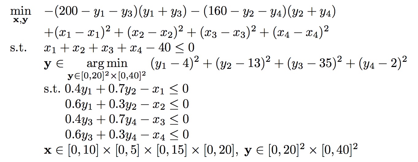
The original formulation of this problem in (Aiyoshi & Shimizu, 1981) involved two independent lower-level problems. We regrouped those two problems so as to form a unique lower-level problem (Colson, 2002).
Optimal solution
| Objective values | Solution points |
|---|---|
| F* = -6600.0 | x* = (7.0, 3.0, 12.0, 18.0) |
| f* = 54.000 | y* = (0.0, 10.0, 30.0, 0.0) |
“Corollary 3 implies that any convex combination of these points is likewise optimal so some ambiguity still exists in the model; however, for any of these points chosen by the leader, the followers’ solutions seem to lie on the efficient frontier” (Bard, 1988).
Sources where this problem occur
Original source:
- Numerical example in (Aiyoshi & Shimizu, 1981)
Other sources:
- Example 2 in (Bard, 1988)
- Bard88Ex2 problem in (Colson, 2002) and in (Colson et al., 2005)
Description of the problem in the AMPL format
set I := {1..4};
set J := {1..4};
param xlb{I};                        # Lower Bounds for the outer variable
param xub{I};                        # Upper Bounds for the outer variable
param ylb{J};                        # Lower Bounds for the inner variable
param yub{J};                        # Upper Bounds for the inner variable
var x{i in I} >= xlb[i], <= xub[i];  # Outer variable
var y{j in J} >= ylb[j], <= yub[j];  # Inner variable
var l{1..12} >= 0, <= 1000;          # KKT Multipliers

minimize outer_obj: -(200 - y[1] - y[3])*(y[1] + y[3]) - (160 - y[2] - y[4])*(y[2] + y[4])
+ (x[1]-x[1])^2 + (x[2]-x[2])^2 + (x[3]-x[3])^2 + (x[4]-x[4])^2;   # Outer objective

subject to
# Inner constraints
    outer_con1: x[1] + x[2] + x[3] + x[4] - 40 <= 0;
# Inner objective:
    inner_obj: (y[1] - 4)^2 + (y[2] - 13)^2 + (y[3] - 35)^2 + (y[4] - 2)^2 = 0;
# Inner constraints
    inner_con1: 0.4*y[1] + 0.7*y[2] - x[1] <= 0;
    inner_con2: 0.6*y[1] + 0.3*y[2] - x[2] <= 0;
    inner_con3: 0.4*y[3] + 0.7*y[4] - x[3] <= 0;
    inner_con4: 0.6*y[3] + 0.3*y[4] - x[4] <= 0;
# KKT conditions:
    stationarity_1:    2*(y[1] - 4) + 0.4*l[1] + 0.6*l[2] - l[5] + l[6] = 0;
    stationarity_2:    2*(y[2] - 13) + 0.7*l[1] + 0.3*l[2] - l[7] + l[8] = 0;
    stationarity_3:    2*(y[3] - 35) + 0.4*l[3] + 0.6*l[4] - l[9] + l[10] = 0;
    stationarity_4:    2*(y[4] - 2) + 0.7*l[3] + 0.3*l[4] - l[11] + l[12] = 0;
    complementarity_1: l[1]*(0.4*y[1] + 0.7*y[2] - x[1]) = 0;
    complementarity_2: l[2]*(0.6*y[1] + 0.3*y[2] - x[2]) = 0;
    complementarity_3: l[3]*(0.4*y[3] + 0.7*y[4] - x[3]) = 0;
    complementarity_4: l[4]*(0.6*y[3] + 0.3*y[4] - x[4]) = 0;
    complementarity_5: l[5]*y[1] = 0;
    complementarity_6: l[6]*(y[1] - 20) = 0;
    complementarity_7: l[7]*y[2] = 0;
    complementarity_8: l[8]*(y[2] - 20) = 0;
    complementarity_9: l[9]*y[3] = 0;
    complementarity_10: l[10]*(y[3] - 40) = 0;
    complementarity_11: l[11]*y[4] = 0;
    complementarity_12: l[12]*(y[4] - 40) = 0;


# Data for parameter bounds
data;
param xlb :=
    1  0
    2  0
    3  0
    4  0
;
param xub :=
    1  10
    2  5
    3  15
    4  20
;
param ylb :=
    1  0
    2  0
    3  0
    4  0
;
param yub :=
    1  20
    2  20
    3  40
    4  40
;
References
- E. Aiyoshi and K. Shimizu, Hierarchical decentralized systems and its new solution by a barrier method, IEEE Transactions on Systems, Man and Cybernetics, (1981), pp. 444-449
- J. F. Bard, Convex two-level optimization, Mathematical Programming, 40 (1988), pp. 15–27
- B. Colson, P. Marcotte, and G. Savard, A trust-region method for nonlinear bilevel programming: algorithm and computational experience, Computational Optimization and Applications, 30 (2005), pp. 211–227
- B. Colson, BIPA(BIlevel Programming with Approximation Methods)(software guide and test problems), Cahiers du GERAD, (2002)
![]()
![]()