b_1991_01v : Linear-Linear problem, variation of b_1991_01
Comments on the problem
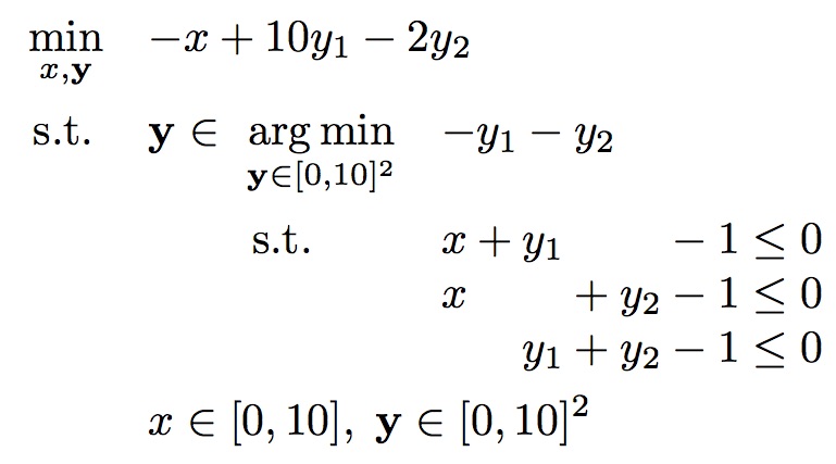
This is a variation of b_1991_01 problem. The only difference is the outer objective function, which is changed from -x + 10*y1 - y2 to -x + 10*y1 - 2y2.
The leader is faced with an ambiguous situation for all choices but one. Only at x = 1 is the follower’s response, y = (0,0), unique. Notice, however, that the point x = 0, y = (0,1) is most preferred by the leader giving F = -2, but may not be realized despite the fact that it is in the inducible region (bilevel feasible region); that is, the follower might very well pick y = (1,0) giving F = 10 for the leader, while keeping unchanged value f = -1 for the follower.
This example suggests that without some incentive, the follower has no reason to select the point y = (0,1) which would be best for the leader.
Optimal solution
| Objective values | Solution points |
|---|---|
| F* = -2.000 | x* = 0.000 |
| f* = -1.000 | y* = (0.000, 1.000) |
Sources where this problem occurs
Original source:
- Analized in Example 15.1.2 in (Shimizu et al., 1997)
Other sources:
- Analized in Example 8.1.2 in (Bard, 1998)
Description of the problem in the AMPL format
var x >= 0, <= 10;         # Outer variable
var y{1..2} >= 0, <= 10;   # Inner variable
var l{1..7} >= 0, <= 10;   # KKT Multipliers

minimize outer_obj: -x + 10*y[1] - 2*y[2];  # Outer objective

subject to
# Inner objective:
    inner_obj: -y[1] - y[2] = 0;
# Inner constraints
    inner_con1:     x + y[1] - 1 <= 0;
    inner_con2:     x + y[2] - 1 <= 0;
    inner_con3:     y[1] + y[2] - 1 <= 0;
# KKT conditions:
    stationarity_1:    -1 + l[1] + l[3] - l[4] + l[5] = 0;
    stationarity_2:    -1 + l[2] + l[3] - l[6] + l[7] = 0;
    complementarity_1: l[1]*(x + y[1] - 1) = 0;
    complementarity_2: l[2]*(x + y[2] - 1) = 0;
    complementarity_3: l[3]*(y[1] + y[2] - 1) = 0;
    complementarity_4: l[4]*y[1] = 0;
    complementarity_5: l[5]*(y[1] - 10) = 0;
    complementarity_6: l[6]*y[2] = 0;
    complementarity_7: l[7]*(y[2] - 10) = 0;
References
- J. F. Bard, Some properties of the bilevel programming problem, Journal of optimization theory and applications, 68 (1991), pp. 371–378
- J. F. Bard, Practical Bilevel Optimization, vol. 30 of Nonconvex Optimization and Its Applications, Springer US, 1998
- Floudas, C. A., Pardalos, P. M., Adjiman, C., Esposito, W. R., Gümüs, Z. H., Harding, S. T., … & Schweiger, C. A. (2013). Handbook of test problems in local and global optimization (Vol. 33). Springer Science & Business Media
- K. Shimizu, Y. Ishizuka, and J. F. Bard, Nondifferentiable and Two-Level Mathematical Programming, vol. 102, Kluwer Academic Publishers, Boston, 1997
![]()
![]()