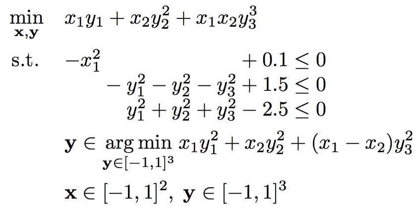
mb_2007_24 : Nonlinear-Nonlinear bilevel problem from [Mitsos & Barton, 2007]
Comments on the problem
Note, that two global optimal solutions exist, while in (Mitsos & Barton, 2007) only one solution was reported. Moreover, the third outer constraint 2.5 + y^2_1 + y^2_2 + y^2_3 <= 0 is always infeasible, as y^2_1 + y^2_2 + y^2_3 >= 0. To make it feasible, we negated the constant term. After this modification, optimal solution point is the same, as was reported in the original source. Note, that the authors in (Nie et al., 2017) fixed this problem in the same way, but have not mentioned in a text.
Sources where this problem occurs
Original source:
- Example 3.26 (mb_2_3_02) in (Mitsos & Barton, 2007)
Other sources:
- mb_2_3_02 in (Mitsos et al., 2008)
- Problem No. 33 from Table 4 in (Kleniati & Adjiman, 2014)
- Example 5.1 in (Nie et al., 2017)
Optimal solution
| Objective values | Solution point(s) | |
| F* = -2.350 | x* = (-1.0,-1.0) | x* = (-1.0,-1.0) |
| f* = -2.000 | y* = (1.0,1.0,-0.707) | y* = (1.0,-1.0,-0.707) |
Description in the AMPL format
var x{1..2} >= -1, <= 1;   # Outer variables
var y{1..3} >= -1, <= 1;   # Inner variables
var l{1..6} >= 0, <= 100;  # Multipliers

minimize outer_obj: x[1]*y[1] + x[2]*y[2]^2 + x[1]*x[2]*y[3]^3;

subject to
# Outer constraints:
    outer_con_1: -x[1]^2 <= -0.1;
    outer_con_2: -(y[1]^2 + y[2]^2 + y[3]^2) <= -1.5;
    outer_con_3: y[1]^2 + y[2]^2 + y[3]^2 <= 2.5;
# Inner objective
    inner_obj: x[1]*y[1]^2 + x[2]*y[2]^2 + (x[1]-x[2])*y[3]^2 = 0;
# KKT conditions
    stationarity_1: 2*x[1]*y[1] -l[1] + l[2] = 0;
    stationarity_2: 2*x[2]*y[2] -l[3] + l[4] = 0;
    stationarity_3: 2*(x[1]- x[2])*y[3] -l[5] + l[6] = 0;
    complementarity_1: -l[1] -l[1]*y[1] = 0;
    complementarity_2: -l[2] + l[2]*y[1] = 0;
    complementarity_3: -l[3] -l[3]*y[2] = 0;
    complementarity_4: -l[4] + l[4]*y[2] = 0;
    complementarity_5: -l[5] -l[5]*y[3] = 0;
    complementarity_6: -l[6] + l[6]*y[3] = 0;
References
- P.-M. Kleniati and C. S. Adjiman, Branch-and-Sandwich: a deterministic global optimization algorithm for optimistic bilevel programming problems. Part II: Convergence analysis and numerical results, Journal of Global Optimization, 60 (2014), pp. 459–481
- A. Mitsos and P. I. Barton, A Test Set for Bilevel Programs, 2007. (Last updated September 19, 2007)
- A. Mitsos, P. Lemonidis, and P. I. Barton, Global solution of bilevel programs with a nonconvex inner program, Journal of Global Optimization, 42 (2008), pp. 475–513
- J. Nie, L. Wang, and J. Ye, Bilevel polynomial programs and semidefinite relaxation methods, SIAM Journal on Optimization, 27 (2017), pp. 1728–1757
![]()
![]()